USCT - design

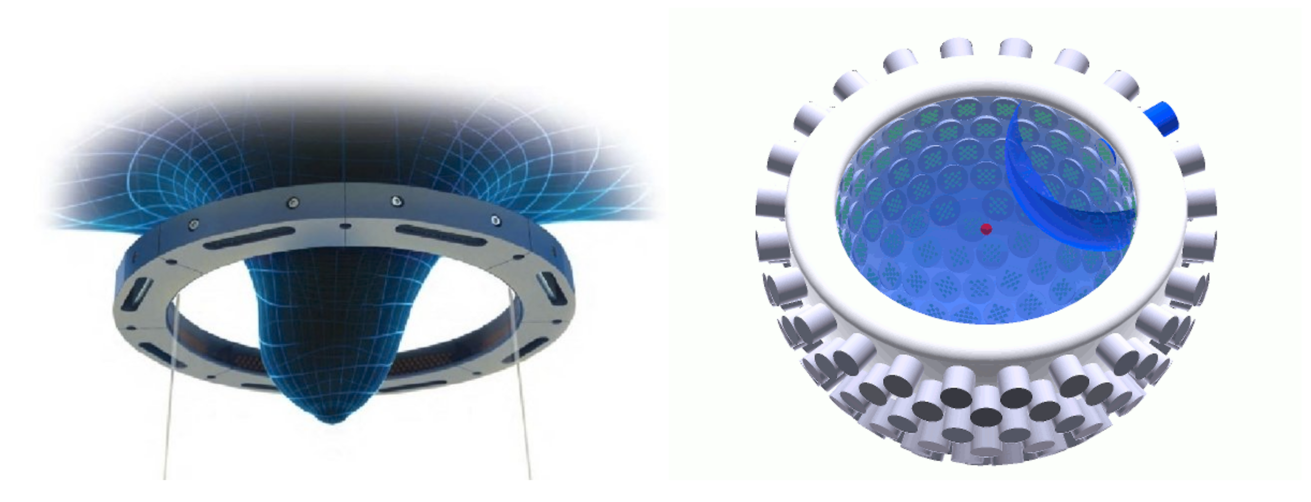
There are mainly two classes of USCT devices depending on the data coverage they provide (see examples in figure below):

(1) Two-dimensional (2D) devices arrange the transducers in a plane (e.g., in a ring-shaped transducer holder) and produce a set of 2D breast images at different elevations. This arrangement is helpful to reduce the dimension of the physical problem and speed up the image reconstruction process. It enables us to use sophisticated tomographic methods (numerically solving the wave equation) that otherwise would be computationally prohibitive to implement. However, fast reconstructions neglect the three-dimensional nature of the wave propagation (e.g., out-of-plane scattering) and introduce artifacts in the final images, reducing their accuracy.

(2) Three-dimensional (3D) devices arrange transducers in a semispherical setup and can provide volumetric tissue images at the expense of a higher acquisition and computational cost. Currently, this cost does not allow the implementation of advanced tomographic methods and significantly limits the spatial resolution of final images.

As we see, USCT designs and tomographic methods are interrelated. My work has focused on developing Optimal Experimental Design (OED) approaches to find the optimal configuration of transducers for commonly applied image reconstruction methods. We define the optimal setup as the configuration of transducers that reduces most uncertainties of reconstructed images post-acquisition. More details can be found in my Ph.D. thesis.

Optimal experimental design

Theoretical background

The goal of USCT is to estimate the acoustic tissue parameters \(\mathbf{m}\) from the observations of the ultrasound signals \(\mathbf{d}\) that are recorded by an experimental setup \(\mathbf{s}\). We can express the physical model relating our observations with unknown tissue properties as \(\mathbf{F}\) as

\begin{equation} \mathbf{d} = \mathbf{F}(\mathbf{m};\mathbf{s}) + \epsilon, \end{equation} where \(\mathbf{F}\) is the forward operator encoding our physical model, and \(\epsilon\) accounts for measurement noise. In USCT, the nonlinearities of \(\mathbf{F}\) with respect to \(\mathbf{m}\) are not too severe, and we typically use linearized forward operators with respect to some prior knowledge about tissue \(\mathbf{m}_p\):

\begin{equation} \mathbf{F}(\mathbf{m};\mathbf{s}) \approx \mathbf{F}(\mathbf{m}_p;\mathbf{s}) + \mathbf{F}’(\mathbf{m}_p;\mathbf{s})(\mathbf{m} - \mathbf{m}_p), \end{equation}

For such linearized problems, we can compute the posterior covariance operator \(\Gamma_\text{post}\). This operator contains the uncertainties in tissue properties that we expect post-reconstruction and is expressed as

\begin{equation} \Gamma_\text{post}(\mathbf{s}) = \left( {\mathbf{F}’(\mathbf{s})}^{T} \Gamma_\text{noise}^{-1}\mathbf{F}’(\mathbf{s}) + \Gamma_\text{prior}^{-1}\right)^{-1}. \end{equation}

Here, \(\Gamma_\text{noise}\) and \(\Gamma_\text{prior}\) are the covariance operator of measurements noise and our prior knowledge about tissue properties, respectively, which we assume to be Gaussian. \(\Gamma_\text{post}\) shows useful properties to measure the quality of an experimental configuration. First, it depends on the parameters that define the experimental setup \(\mathbf{s}\). This allows us to compare different candidates and select the ones that give the lowest uncertainties in the parameter estimation. Second, it neither depends on the observations nor the unknown model parameters, which means that it could be used to optimize the experiment before any realization. Last, it shows the same structure for any forward operator, under the condition that these are linear or can be linearized with respect to the model parameters. This allows us to present general formulations of the OED problem, independent of the tomographic method that is intended to be applied post-acquisition.

Optimal experimental design approach

Assume that \(\Theta\) is a scalar function that quantifies the level of expected uncertainties in the parameters by extracting some properties from \(\Gamma_\text{post}\). Then, we can formulate the OED problem as a minimization problem

\begin{equation}\label{eq:OED} \min_{\mathbf{s} \in \mathcal{S}} \Theta \left(\Gamma_\text{post}\right), \end{equation}

where \(\mathcal{S}\) represents the space for all possible experimental configurations. In our work, we define \(\Theta\) as the determinant of the posterior covariance matrix

\begin{equation}\label{eq:D-optLog} \Theta = \log \det \left(\Gamma_\text{post} \ \right). \end{equation}

The determinant corresponds to the product of the eigenvalues of \(\Gamma_\text{post}\), and thus, we minimize the volume of the uncertainty ellipsoid in the estimated tissue parameters. From information theory, this quantity can be related to the expected information gain.

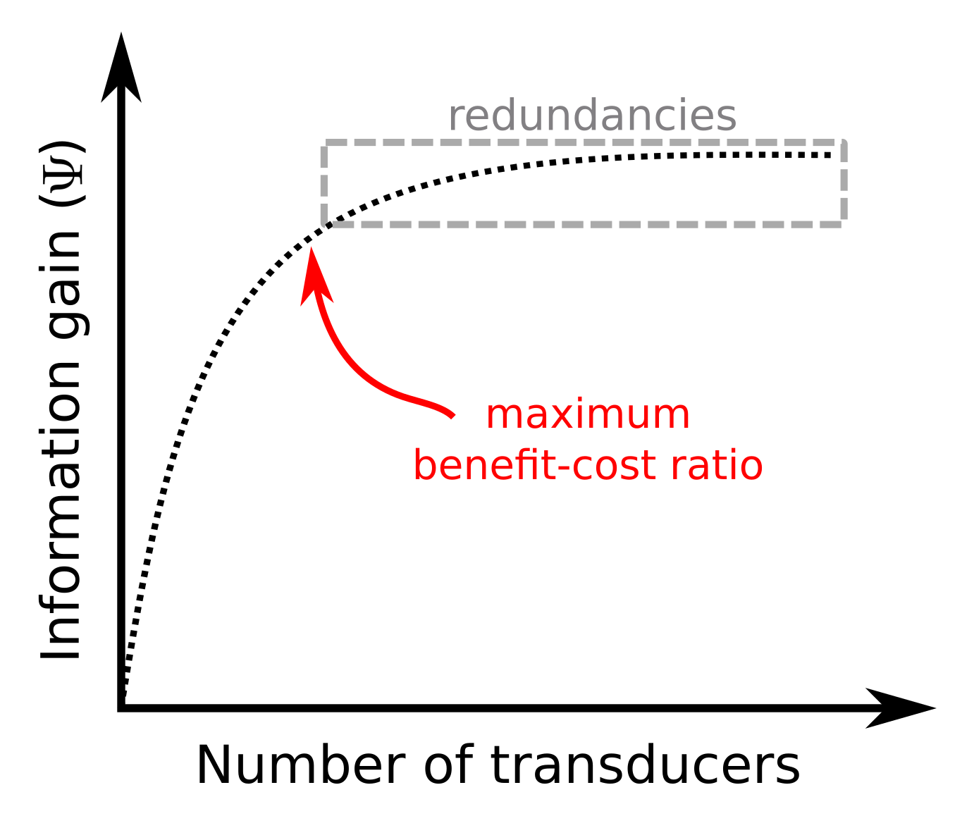
To optimize the experimental setup in USCT, we use a sequential approach. We start from an experimental configuration that considers all candidate transducers active, and we deactivate them one by one in each iteration. This approach has the advantage of providing benefit-cost curves that illustrate the gain in the data information content with respect to the experimental cost:

The benefit-cost curve is particularly useful maximize the benefit-cost ratio of the experiment by identifying redundancies in our observations.

Examples

Here we show few results to illustrate the benefit of optimally designing an experiment. We consider the experimental data that was provided as part of the SPIE USCT Data Challenge 2017 by the Spanish National Research Council (CISC) and the Complutense University of Madrid (the data can be found here). The setup consists of two transducer arrays of 16 elements. The transducers in one array act as emitters whereas the ones in the other array are recording. The receiving array is always located opposite to the emitting array, and the whole the whole system is rotated into 23 different positions, describing a circle with radius 95 mm. Receivers record signals that travel through a tissue mimicking phantom based on water, gelatine, graphite powder, and alcohol. The phantom has a cylindrical homogeneous background with a diameter of 94 mm, two inclusions of 2 cm diameter (lower and higher speed of sound than the background), and two steel needles.

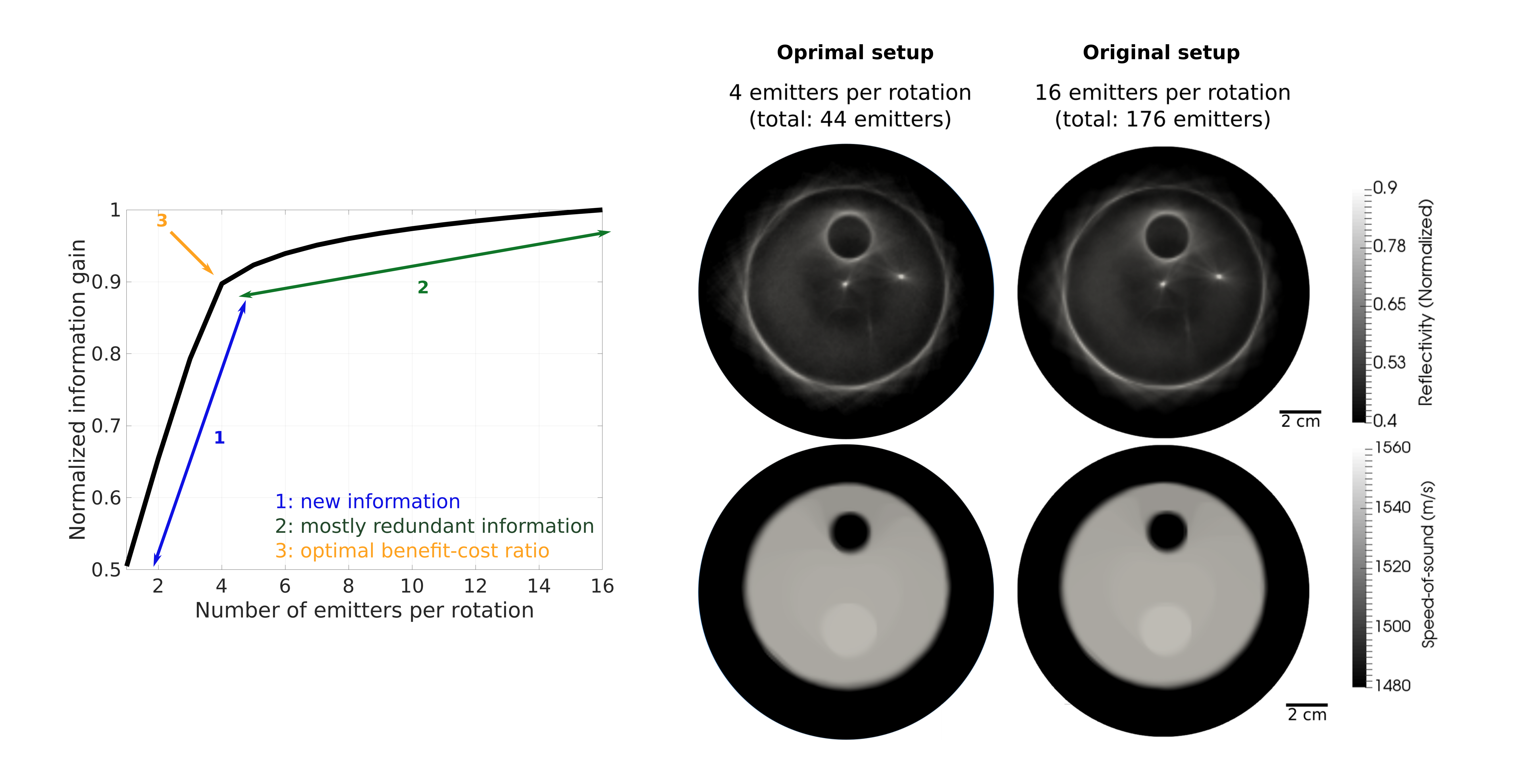
Our goal is to decrease the data volume to reduce the time to solution. Here, the number of measurements is mainly controlled by the total number of emitting elements in the transducer array. We therefore aim to select the most informative ones, removing those that provide redundant information about the phantom. After applying our OED algorithm, we obtain the following result for the reconstruction of phantom speed of sound and reflectivity:

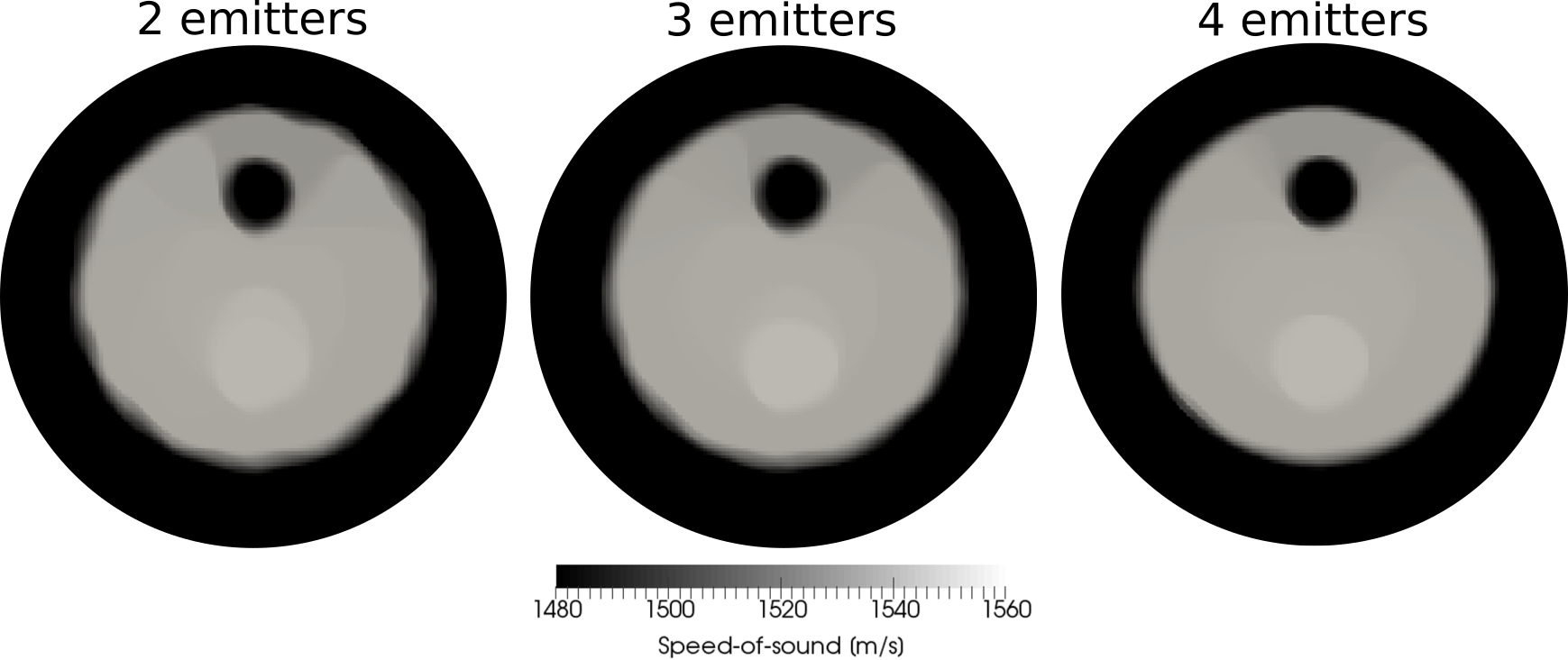
To understand the meaning of the benefit-cost curve, we show the speed-pf-sound reconstructions that we acquire for different number of emitters:

For the experimental data used in this example, we could speed-up by four the acquisition and reconstruction time by optimally designing the experiment, without losing relevant information about the tissue. That is, in this example, 75% of the data is redundant!

The benefit of an optimized USCT system, in terms of the image quality and computational resources, for clinical practice is tremendous. Once the acquisition system is optimized, the impact of the reduced cost in the recursive use of the scanning system may become very significant.